The following is a brief tutorial written for my students on grabbing FITS images from the Sloan Digitial Sky Survey then loading and displaying them in python using tools from the Astropy Project. It should make for a good test case.
Everything below this point is an IPython notebook and can be downloaded here, or viewed statically here.
Viewing and manipulating FITS images in Python
This notebook started life as a tutorial on the astropy tutorials page, and was originally written by Lia R. Corrales.
We'll need to import some basic modules to do this; note that %matplotlib inline causes images to appear in the notebook.
import numpy as np
import matplotlib as mpl
import matplotlib.pyplot as plt
%matplotlib inline
In order to handle FITS images in python, we'll need the fits module from astropy:
from astropy.io import fits
The following is optional, and will only work if you have Seaborn installed on your machine, but is a significant improvement over the matplotlib defaults.
import seaborn as sns
sns.set_context('poster')
sns.set_style('white')
Downloading the data
Go to the SDSS website and download the image of your choice from the SDSS catalog. Here we'll use M42, the Orion Nebula, which looks like this:
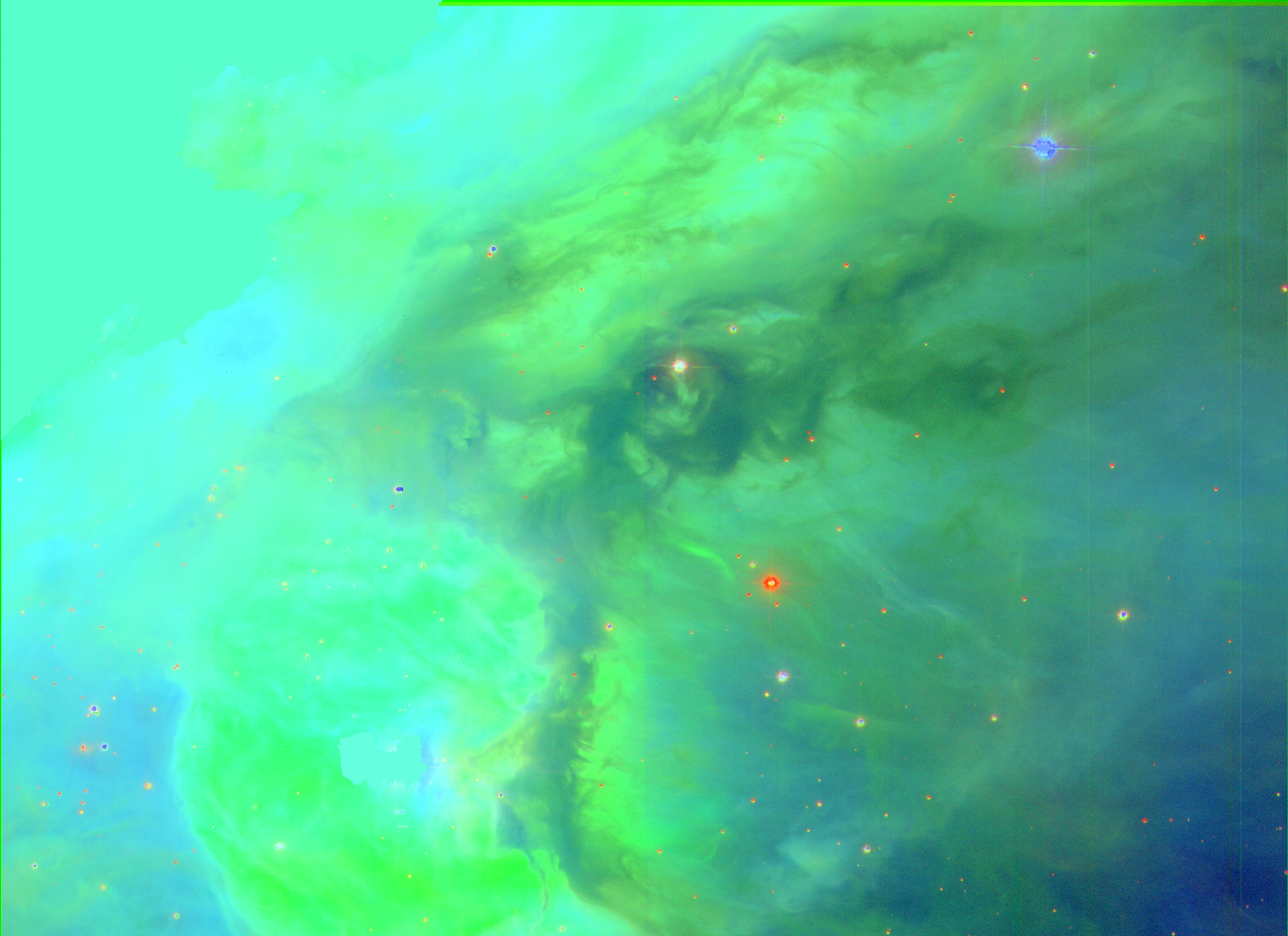
You will need to unzip the files!!! The FITS images you download will be compressed (with a .gz or .bz2 extension). You'll need to extract the file using the program of your choice before proceeding.
Make sure you're in the correct directory (on your machine):
pwd
ls
ls data
Notice how all of the fits files have that .bz2 extension. We'll need to extract them to proceed.
ls data
Having extracted the uncompressed fits files, we are now ready to proceed.
Opening FITS files and loading the image data
Let's open the g-band FITS file and find out what it contains.
hdu_list = fits.open("data/frame-g-006073-4-0063.fits")
hdu_list.info()
Generally the image information is located in the PRIMARY block. The blocks are numbered and can be accessed by indexing hdu_list.
image_data = hdu_list[0].data
You data is now stored as a 2-D numpy array. Want to know the dimensions of the image? Just look at the shape of the array.
print(type(image_data))
print(image_data.shape)
At this point, we can just close the FITS file. We have stored everything we wanted to a variable.
hdu_list.close()
SHORTCUT
If you don't need to examine the FITS header, you can call fits.getdata to bypass the previous steps.
image_data = fits.getdata("data/frame-g-006073-4-0063.fits")
print(type(image_data))
print(image_data.shape)
Let's get some basic statistics about our image
print('Min:', np.min(image_data))
print('Max:', np.max(image_data))
print('Mean:', np.mean(image_data))
print('Stdev:', np.std(image_data))
Viewing the image
plt.imshow(image_data, cmap='afmhot', origin='lower')
plt.colorbar()
# To see more color maps go to http://wiki.scipy.org/Cookbook/Matplotlib/Show_colormaps

Unforturnately, we can't really see much here because of the color range. Lets adjust that manually and see what happens.
plt.imshow(image_data, cmap='afmhot', origin='lower')
plt.clim(0,30)

Play around with the color limits until you find the best range of values. Looking at the x-range of the histogram below will help you get some idea where most of the dynamic range of the image is. In this image it's all near, but greater than 0. That won't necessarily be the case for all images.
Plotting a histogram
To make a histogram with matplotlib.pyplot.hist(), you need to cast the data from a 2-D to array to something one dimensional.
Here we'll use the iterable python object image_data.flat.
print(type(image_data.flat))
NBINS = 1000
with sns.axes_style("darkgrid"):
    histogram = plt.hist(image_data.flat, NBINS)

Displaying the image with a logarithmic scale
When looking at images with a large dynamic range, it is often useful to rescale the image. Logarithmic scaling basically does this to the pixel counts:
NBINS = 1000
with sns.axes_style("darkgrid"):
    histogram = plt.hist(image_data.flat, NBINS)
    plt.yscale('log', nonposy='clip') #Same histogram, just with logarithmic scaling on the y-axis.

To get a logarithmically scaled image, we need to load the LogNorm object from matplotlib.
from matplotlib.colors import LogNorm
plt.imshow(image_data, cmap='afmhot', norm=LogNorm(), origin='lower')
